In the last century discrete mathematics has developed tremendously and many of these fields have revealed themselves to be particularly effective, and elegantly simple, in instances where their continuous counterparts either weren't appropriate or remain virtually as complicated and convoluted as the phenomena they aim to explain. In this vein, we apply tools from graph theory and cellular automata theory to study generalized neuropercolation models for the sake of ultimately creating biologically inspired AI.

In this part of the project, we focus particularly on a neural network model, \( N(E,I) \), with coupled excitatory, \(E\), and inhibitory, \(I\), layers. Both \(E\) and \(I\) can be represented as graphs with vertices that take on one of two states: active or inactive. The state that a vertex takes in either layer at any given time is fully dependant on their neighbors. In what follows we briefly describe \(N(E,I)\) and the rules that guide its evolution through time, for a full account and rigorous treatment we refer the reader to the sources cited below.

The excitatory layer, \(E\), is defined as the Erdős-Rényi random graph \(G_{\mathbb{Z}^2_N,p_d}\). In other words \(E\) is a graph with all of the vertices and edges of a \(\mathbb{Z}^2\) lattice over an \(N \times N\) grid, with boundary conditions (note that this can be thought of as the torus \(\mathbb{T}^2 = (\mathbb{Z}/N\mathbb{Z})^2\)), in addition to random edges that are added with a probability that is inversely proportional to the graph distance between vertices. The inhibitory layer, \(I\), is a fully connected graph with one vertex for every four vertices in \(E\). The layers are coupled by a surjective mapping from \(E\) onto \(I\) where every four vertices in \(E\) are mapped to exactly one vertex in \(I\). Together these layers fully describe the structure of \(N(E,I) \).

The state of every vertex in the network is updated at each step in time. The state of vertices in both \(E\) and \(I\) are determined in slightly different ways. A vertex in \(E\) is active if \(k\) or more of the vertices in its closed neighborhood are active, where \(k\) is a positive integer. Otherwise that vertex is said to be inactive. A vertex in \(I\) is said to be active if \(\ell\) or more of the excitatory vertices mapped to it are active, where \(\ell\) is a positive integer. Otherwise that vertex is inactive. As one might expect from their names, the vertices in \(E\) and \(I\) heavily influence one another. The inhibitory layer, \(I\), passively activates along with \(E\) until the number of active inhibitory vertices surpasses a predefined threshold, \(m \in [0, \frac{N^2}{4}]\), and fires. At the moment of firing both layers experience a sudden change in activity; all of the currently active inhibitory vertices become inactive along with all of the excitatory vertices that are mapped to said inhibitory vertices.

To see this in action, refer to the following video(Video 1). Here the excitatory layer has \(N^2 = 10,000\) vertices and no additional edges were added onto the lattice structure. We leave the inhibitory layer unseen because we chose the mapping from \(E\) onto \(I\) at random and assign \(k=2, \ell=4,\) and \(m=2100\).

As one can imagine any variations in \(k, \ell, m, N,\) the neighborhoods of vertices in \(E\), and the mapping from \(E\) onto \(I\) drastically change the behaviour we observe from the network.

Of particular interest to us is the oscillatory behaviour that arises from the interplay between \(E\) and \(I\). The figure below(Figure 1) encapsulates this particularly well and was produced from data gather by running simulations like what was seen in the video above. We held fixed \(N=100\), \(k=2\), \(l=4\), mapped \(E\) to \(I\) at random in each experiment, and ran the simulations with varying initial excitatory activation densities and values of \(m\). After \(1000\) time steps of each simulation we stored the length of time between the last two firings of the inhibitory layer. With that in mind, the horizontal axis represents the values of \(m\), the vertical axis represents the initialization density, and the color of each cell represents the \(log_2\) of the last oscillation time.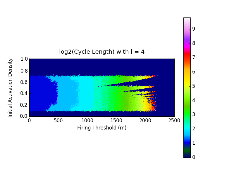

Note the fractal like behaviour at the higher values of \(m\), the rather sharp cutoff of oscillation formation at \(\approx 0.1\) and \(\approx 0.7\) initialization densities, and the apparent independence of period length from initialization density. All of this only begins to describe the fascinating dynamical behaviour that the system displays. When these simulations are run for significantly longer than just the \(1000\) time steps expressed in this figure, we see that the behaviour at specific ranges of \(m\) render this figure a very rough approximation of the true oscillatory behaviour in the network. Furthermore as we change the neighborhoods of excitatory vertices, gradually adding edges, we are reminded that the depth displayed by this system doesn't disappoint. In the figure below(Figure 2) we have essentially taken the outline of the fractal like shape above, but with varying degrees of bolstering the neighborhood of vertices. The parameter denoted as \(\lambda\) can be thought of as describing "on average \(\lambda\) new neighbors are added to each vertex".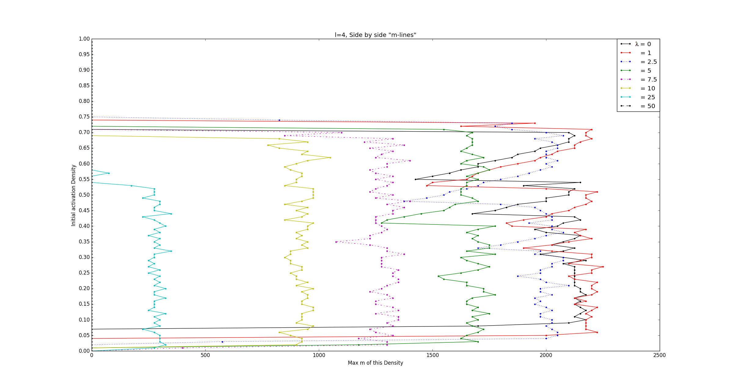

By plotting these in three dimensions(Figure 3) we further notice that the fractal like indents found at differing levels of connectivity are in fact one and the same, despite appearing at different initialization densities.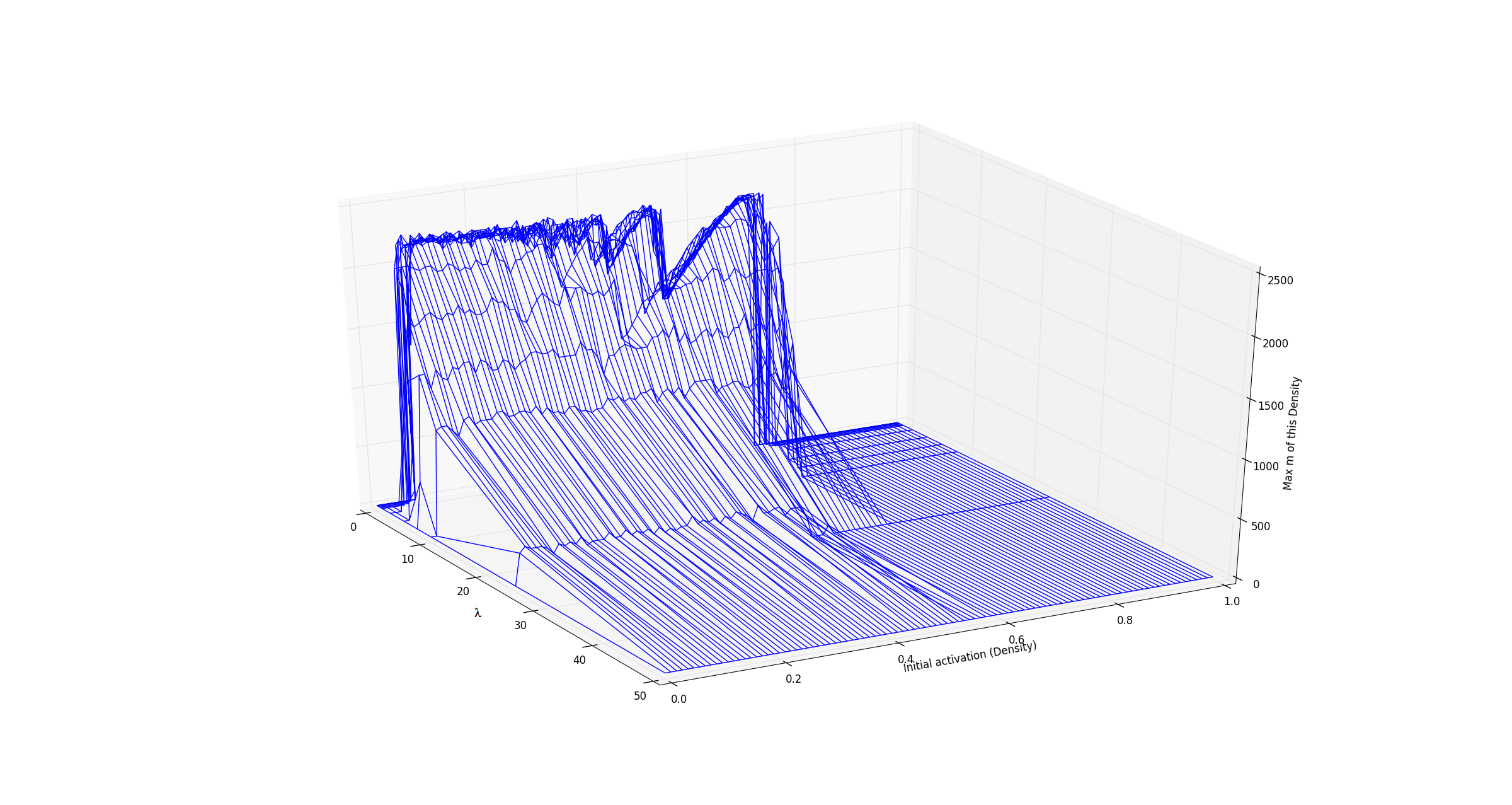

Much of the behaviour in these models remains to be completely understood. With the presence of oscillatory and complicated dynamical behaviour we are led to explore the meaning and nature of chaos. As is the case with most cellular automata, little is understood about the global behaviour that arises from local changes and vice verse. The robustness of the oscillatory behaviors is reminiscent of physiological phenomena that play a key role in multiple functions of the brain (e.g memory). These are among the numerous questions that are at the intersection of philosophy, neuroscience, computer science, and mathematics that we strive to understand.